HOLISMOKES. IV. Efficient mass modeling of strong lenses through deep learning

We present in this paper a convolutional neural network (CNN) to model strong gravitational lenses in the galaxy-galaxy regime. The network is trained on mock images of size 10.75"x10.75" in five filters grizy, which we generate with our own routine. Since it is very important to have training data that are as realistic as possible, we use real observed images of galaxies and only simulate the lensing effect. For this project, the images of the lens' galaxies are from the Hyper Suprime-Cam Survey (HSC) and used in combination with the redshift and velocity dispersion from SDSS. The unlensed images of the sources are taken from the Hubble Ultra Deep Field (HUDF) where also redshifts are available. The simulation code calculates and 'paint' the lensed source on top of the lens image and save the five lens mass parameters of the Singular Isothermal Ellipsoid (SIE) profile. The routine, which was also used in H0LISMOKES II and will be used in upcoming papers of this series, is independent of the image quality and has many user specific options implemented. An overview of the procedure is shown in the following Figure.

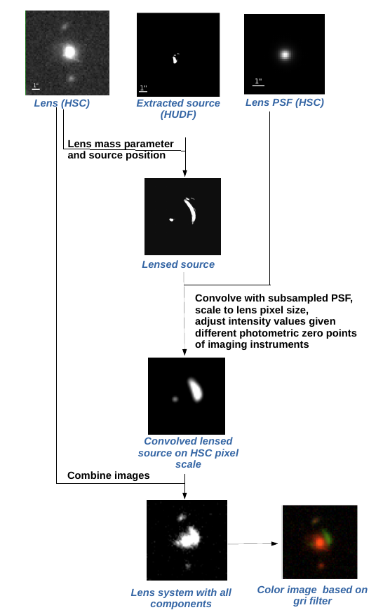
While this routine assumes a parameterization of the SIE profile with axis ratio and position angel, we convert them into a complex ellipticity e_x and e_y for the training as the network seem to have problems with the 2pi modulo position angle. This is in agreement with Hezaveh et al. (2017) and Pearson et al. (2019).

During our network testing, where we did a grid search over the hyper parameters and also considered different network architectures by varying e.g., the number of layers, we found that the distribution of Einstein radii in the training set is very important, especially as this is a key parameter of the model. Therefore, we trained a network under the assumption of different underlying data sets, for example a lower limit of the Einstein radius for the simulations or a different distribution of Einstein radii. We further tested the network performance by limiting to a specific configuration (i.e., only doubles or quads).

We finally present and discuss three different networks in detail:
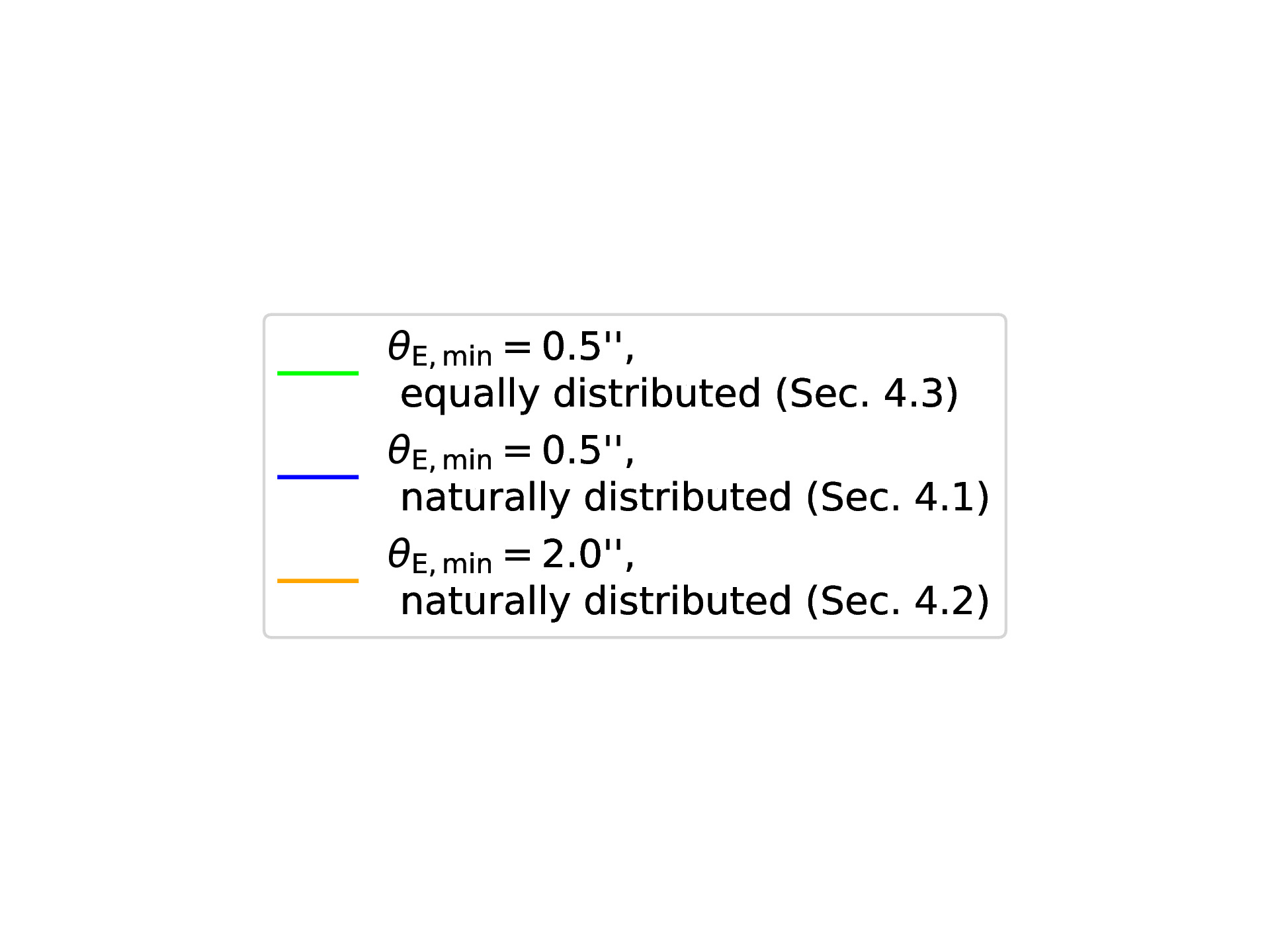
- Naturally distributed Einstein radii with lower limit 0.5"
- Naturally distributed Einstein radii with lower limit 2.0"
- Uniformly distributed Einstein radii with lower limit 0.5"

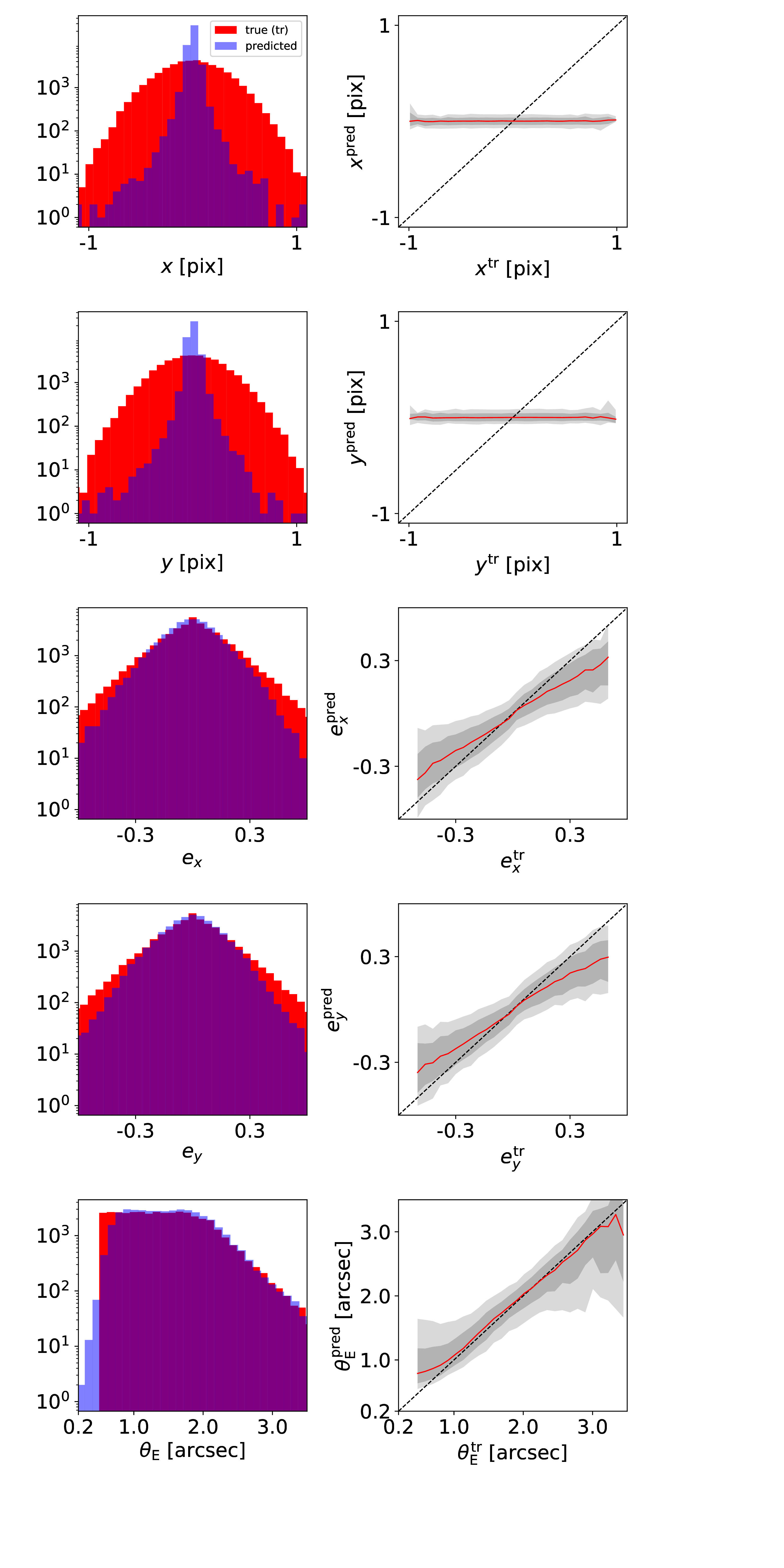
From those three networks we favor the last one because of its wide Einstein radius range and better performance for images with higher (θ_E~2-4") image separation. The following figure shows the performance of this specific network, and in detail on the left panel histograms of the ground truth (red) and of the predicted values (blue). The right panel shows a direct comparison of the predicted against the true value, where the red line indicates the median of the distribution and the gray bands give the 1σ (16th to 84th percentile) and 2σ ( 2.5th to 97.5th percentile) ranges. From top to bottom are the five different model parameters, lens center x and y, complex ellipticity e_x and e_y , and Einstein radius θ_E.

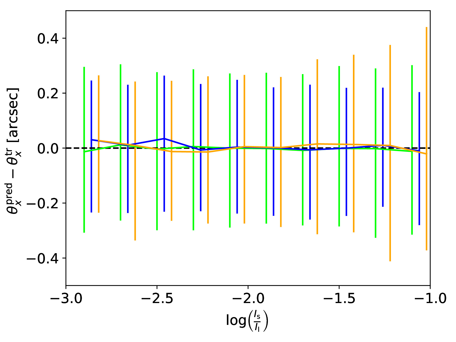
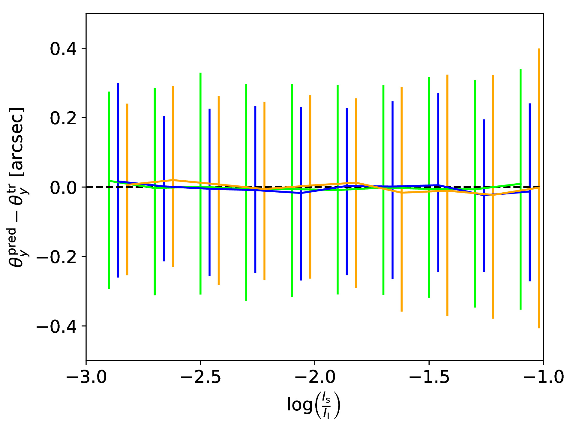
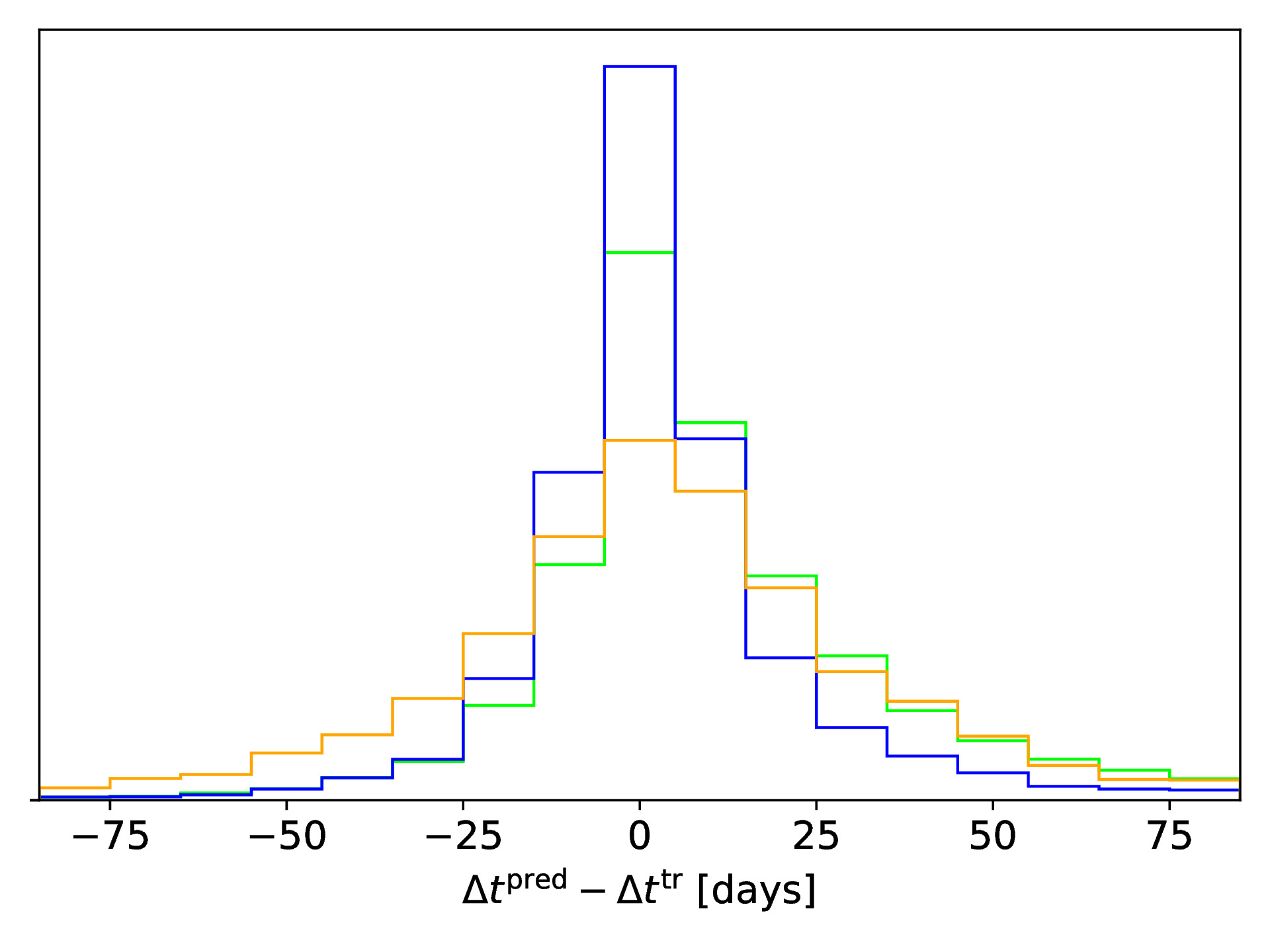
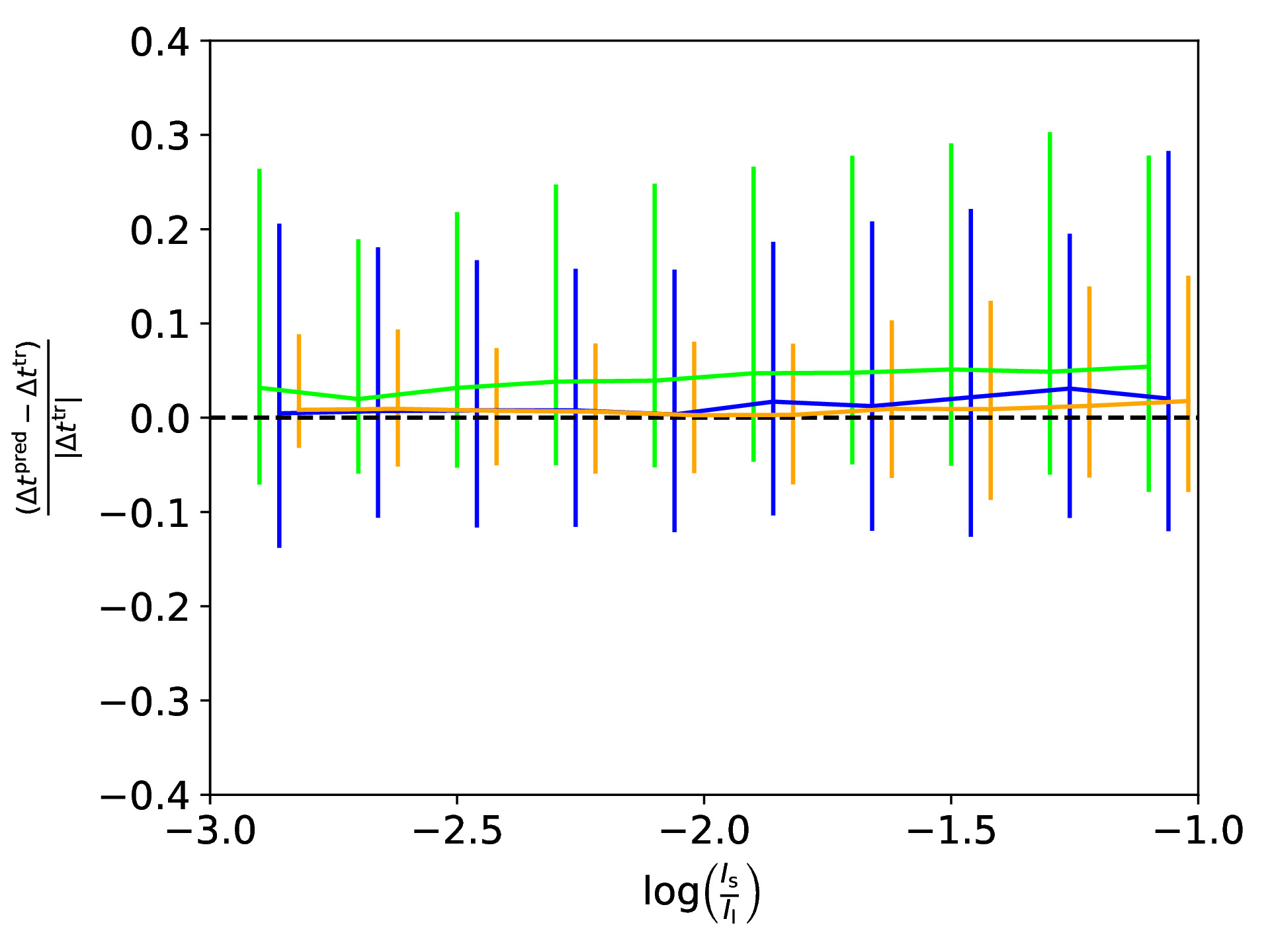
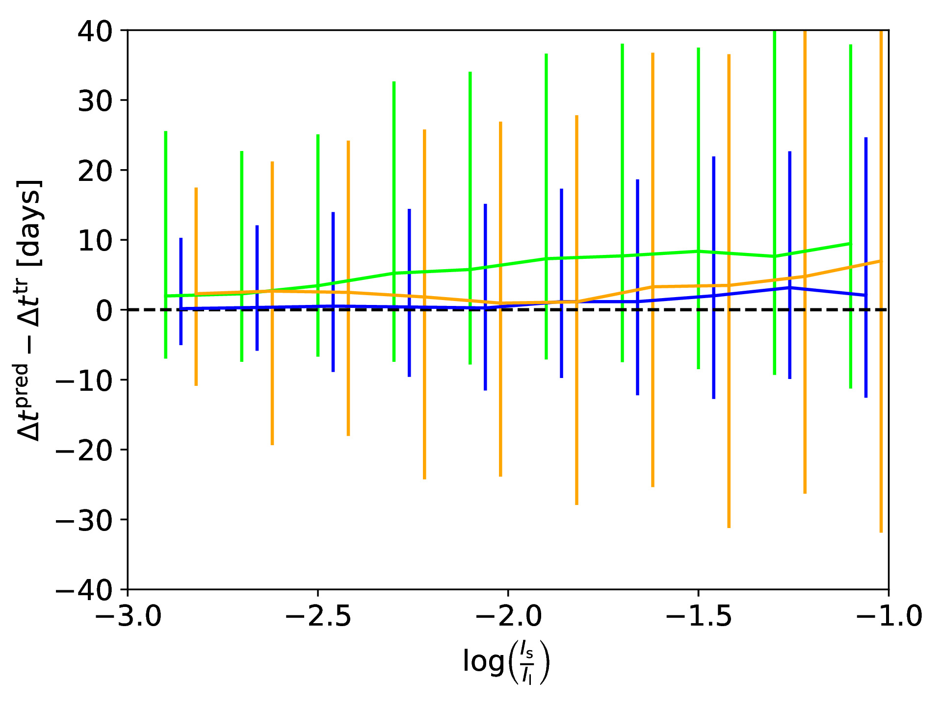
If a supernova (SN) would now explode in the source galaxy and would be strongly lensed as well, we can use our SIE mass model obtained with the CNN to predict the location and time for the next appearing image of the strongly lensed SN. To test the accuracy of our obtained model, we use the ground truth to predict the true image positions and time delays, and compare to those calculated based on the CNN predicted SIE mass model. The following figure shows in the top row the difference between true and predicted image positions for x (left panel) and y (right panel) coordinate as a function of the brightness ratio, which is defined as $\mathrm{log(}\frac{\mathrm{I_s}}{\mathrm{I_l}}\mathrm{)}$ with I_s as sum of the lensed source intensity and I_l as sum of the lens intensity. We also show the 1-sigma bars with a slight offset for better visibility. The middle row shows the legend (left panel) and a histogram of the difference in time delays (right panel). The bottom row shows the fractional time delay difference (left panel) and time delay difference (right panel) both again as function of the brightness ratio.

In this paper, we present a neural network to predict the five parameters of the SIE model within fractions of a second with comparable good accuracy. We further show the possibility of using the obtained model to predict the image position and time delays with a reasonable precision given the assumed profile and ground based image quality.